3D FM Example
[1]:
%matplotlib inline
import numpy as np
import warnings
warnings.filterwarnings('ignore')
import plotly.graph_objects as go
[1]:
# import sys
# sys.path.append("../../src/")
[3]:
%load_ext autoreload
%autoreload 2

from qeview.qe_analyse_FM import qe_analyse_FM
import qeview.wannier_loader as wnldr
[4]:
Ang2Bohr = 1.8897259886
Bohr2Ang = 1./Ang2Bohr
QE Analysis
[5]:
calc = qe_analyse_FM('./', 'FeCl2')
Unit Cell Volume:   66.6024  (Ang^3)
alat 6.4228
Reciprocal-Space Vectors cart (Ang^-1)
[[ 1.7853615074 -1.0307789469  0.3372927535]
 [ 0.            2.0615578938  0.3372927535]
 [-1.7853615074 -1.0307789469  0.3372927535]]
Reciprocal-Space Vectors cart (2 pi / alat)
[[ 1.8250245048 -1.0536783891  0.3447859372]
 [ 0.            2.1073567783  0.3447859372]
 [-1.8250245048 -1.0536783891  0.3447859372]]
Real-Space Vectors cart (Ang)
[[ 1.7596395131 -1.0159283466  6.2094281022]
 [ 0.            2.0318566932  6.2094281022]
 [-1.7596395131 -1.0159283466  6.2094281022]]
Real-Space Vectors cart (alat)
[[ 0.2739689241 -0.1581760321  0.9667834369]
 [ 0.            0.3163520641  0.9667834369]
 [-0.2739689241 -0.1581760321  0.9667834369]]


 positions cart (alat)
['Fe', 'Cl', 'Cl']
[[-0.            0.           -0.          ]
 [ 0.           -0.            2.1508692713]
 [ 0.           -0.            0.7494810395]]
positions (frac or crystal)
[[-0.            0.            0.          ]
 [ 0.7415894774  0.7415894774  0.7415894774]
 [ 0.2584105226  0.2584105226  0.2584105226]]
positions (AA)
[[-0.            0.           -0.          ]
 [ 0.           -0.           13.8145396238]
 [ 0.           -0.            4.8137446827]]
[7]:
calc.get_band_structure(bands_up_name=None, bands_dn_name=None, qe_dir='qe')
calc.get_sym_points(filename='band.in')
[8]:
_,_ = calc.get_qe_kpathBS(filename="kpath_qe2.dat", saveQ=True, points_per_unit=20)
G 0.00000000 0.00000000 0.00000000 0.00000000
. 0.05000000 0.05000000 0.05000000 0.05171789
. 0.10000000 0.10000000 0.10000000 0.10343578
. 0.15000000 0.15000000 0.15000000 0.15515367
. 0.20000000 0.20000000 0.20000000 0.20687156
. 0.25000000 0.25000000 0.25000000 0.25858945
. 0.30000000 0.30000000 0.30000000 0.31030734
. 0.35000000 0.35000000 0.35000000 0.36202523
. 0.40000000 0.40000000 0.40000000 0.41374312
. 0.45000000 0.45000000 0.45000000 0.46546102
T 0.50000000 0.50000000 0.50000000 0.51717891
. 0.51382328 0.48617672 0.50000000 0.56763454
. 0.52764655 0.47235345 0.50000000 0.61809018
. 0.54146983 0.45853017 0.50000000 0.66854582
. 0.55529311 0.44470689 0.50000000 0.71900146
. 0.56911639 0.43088361 0.50000000 0.76945710
. 0.58293966 0.41706034 0.50000000 0.81991274
. 0.59676294 0.40323706 0.50000000 0.87036838
. 0.61058622 0.38941378 0.50000000 0.92082402
. 0.62440949 0.37559051 0.50000000 0.97127966
. 0.63823277 0.36176723 0.50000000 1.02173530
. 0.65205605 0.34794395 0.50000000 1.07219094
. 0.66587933 0.33412067 0.50000000 1.12264658
. 0.67970260 0.32029740 0.50000000 1.17310221
. 0.69352588 0.30647412 0.50000000 1.22355785
. 0.70734916 0.29265084 0.50000000 1.27401349
. 0.72117243 0.27882757 0.50000000 1.32446913
. 0.73499571 0.26500429 0.50000000 1.37492477
. 0.74881899 0.25118101 0.50000000 1.42538041
. 0.76264227 0.23735773 0.50000000 1.47583605
. 0.77646554 0.22353446 0.50000000 1.52629169
. 0.79028882 0.20971118 0.50000000 1.57674733
. 0.80411210 0.19588790 0.50000000 1.62720297
H2 0.81793537 0.18206463 0.50000000 1.67765861
. 0.77251604 0.13004616 0.45458066 1.72883931
. 0.72709670 0.07802770 0.40916132 1.78002002
. 0.68167736 0.02600923 0.36374198 1.83120073
. 0.63625802 -0.02600923 0.31832264 1.88238144
. 0.59083868 -0.07802770 0.27290330 1.93356214
. 0.54541934 -0.13004616 0.22748396 1.98474285
H0 0.50000000 -0.18206463 0.18206463 2.03592356
. 0.50000000 -0.16805965 0.16805965 2.08704239
. 0.50000000 -0.15405468 0.15405468 2.13816122
. 0.50000000 -0.14004971 0.14004971 2.18928005
. 0.50000000 -0.12604474 0.12604474 2.24039888
. 0.50000000 -0.11203977 0.11203977 2.29151771
. 0.50000000 -0.09803480 0.09803480 2.34263655
. 0.50000000 -0.08402983 0.08402983 2.39375538
. 0.50000000 -0.07002486 0.07002486 2.44487421
. 0.50000000 -0.05601988 0.05601988 2.49599304
. 0.50000000 -0.04201491 0.04201491 2.54711187
. 0.50000000 -0.02800994 0.02800994 2.59823070
. 0.50000000 -0.01400497 0.01400497 2.64934953
L 0.50000000 0.00000000 0.00000000 2.70046836
. 0.47619048 0.00000000 0.00000000 2.75131065
. 0.45238095 0.00000000 0.00000000 2.80215293
. 0.42857143 0.00000000 0.00000000 2.85299521
. 0.40476190 0.00000000 0.00000000 2.90383749
. 0.38095238 0.00000000 0.00000000 2.95467977
. 0.35714286 0.00000000 0.00000000 3.00552205
. 0.33333333 0.00000000 0.00000000 3.05636434
. 0.30952381 0.00000000 0.00000000 3.10720662
. 0.28571429 0.00000000 0.00000000 3.15804890
. 0.26190476 0.00000000 0.00000000 3.20889118
. 0.23809524 0.00000000 0.00000000 3.25973346
. 0.21428571 0.00000000 0.00000000 3.31057574
. 0.19047619 0.00000000 0.00000000 3.36141803
. 0.16666667 0.00000000 0.00000000 3.41226031
. 0.14285714 0.00000000 0.00000000 3.46310259
. 0.11904762 0.00000000 0.00000000 3.51394487
. 0.09523810 0.00000000 0.00000000 3.56478715
. 0.07142857 0.00000000 0.00000000 3.61562943
. 0.04761905 0.00000000 0.00000000 3.66647171
. 0.02380952 0.00000000 0.00000000 3.71731400
G 0.00000000 0.00000000 0.00000000 3.76815628
. 0.01420968 -0.01420968 0.00000000 3.82002231
. 0.02841936 -0.02841936 0.00000000 3.87188833
. 0.04262904 -0.04262904 0.00000000 3.92375436
. 0.05683872 -0.05683872 0.00000000 3.97562039
. 0.07104840 -0.07104840 0.00000000 4.02748641
. 0.08525808 -0.08525808 0.00000000 4.07935244
. 0.09946776 -0.09946776 0.00000000 4.13121847
. 0.11367744 -0.11367744 0.00000000 4.18308450
. 0.12788712 -0.12788712 0.00000000 4.23495052
. 0.14209680 -0.14209680 0.00000000 4.28681655
. 0.15630648 -0.15630648 0.00000000 4.33868258
. 0.17051616 -0.17051616 0.00000000 4.39054861
. 0.18472584 -0.18472584 0.00000000 4.44241463
. 0.19893552 -0.19893552 0.00000000 4.49428066
. 0.21314520 -0.21314520 0.00000000 4.54614669
. 0.22735488 -0.22735488 0.00000000 4.59801272
. 0.24156455 -0.24156455 0.00000000 4.64987874
. 0.25577423 -0.25577423 0.00000000 4.70174477
. 0.26998391 -0.26998391 0.00000000 4.75361080
. 0.28419359 -0.28419359 0.00000000 4.80547682
. 0.29840327 -0.29840327 0.00000000 4.85734285
. 0.31261295 -0.31261295 0.00000000 4.90920888
. 0.32682263 -0.32682263 0.00000000 4.96107491
S0 0.34103231 -0.34103231 0.00000000 5.01294093
. 0.39402154 -0.28419359 0.05683872 5.07097504
. 0.44701077 -0.22735488 0.11367744 5.12900914
. 0.50000000 -0.17051616 0.17051616 5.18704324
. 0.55298923 -0.11367744 0.22735488 5.24507734
. 0.60597846 -0.05683872 0.28419359 5.30311144
S2 0.65896769 0.00000000 0.34103231 5.36114554
. 0.64451608 0.00000000 0.35548392 5.41389462
. 0.63006447 0.00000000 0.36993553 5.46664370
. 0.61561286 0.00000000 0.38438714 5.51939278
. 0.60116126 0.00000000 0.39883874 5.57214185
. 0.58670965 0.00000000 0.41329035 5.62489093
. 0.57225804 0.00000000 0.42774196 5.67764001
. 0.55780643 0.00000000 0.44219357 5.73038909
. 0.54335482 0.00000000 0.45664518 5.78313816
. 0.52890322 0.00000000 0.47109678 5.83588724
. 0.51445161 0.00000000 0.48554839 5.88863632
F 0.50000000 0.00000000 0.50000000 5.94138539
[9]:
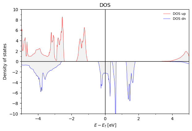
calc.plot_FullDOS()
Energies and DOS were not initialized. I run get_full_DOS
efermi 5.70
[10]:
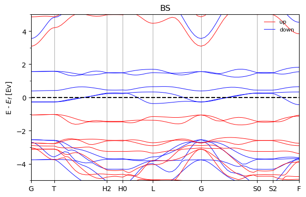
calc.plot_BS(efrom=-5, eto=5)
[11]:
calc.print_bands_range(7, 20)
efermi 5.70
-------------SPIN UP---------------
band 8 eV from  -0.00 to  0.63                 eV-eF from  -5.70 to  -5.07
band 9 eV from  0.14 to  0.77                 eV-eF from  -5.56 to  -4.93
band 10 eV from  0.74 to  2.59                 eV-eF from  -4.96 to  -3.12
band 11 eV from  0.97 to  2.59                 eV-eF from  -4.73 to  -3.12
band 12 eV from  1.17 to  2.67                 eV-eF from  -4.53 to  -3.04
band 13 eV from  2.33 to  2.83                 eV-eF from  -3.38 to  -2.87
band 14 eV from  2.79 to  3.17                 eV-eF from  -2.91 to  -2.53
band 15 eV from  2.92 to  3.29                 eV-eF from  -2.79 to  -2.41
band 16 eV from  4.05 to  4.68                 eV-eF from  -1.66 to  -1.03
band 17 eV from  4.26 to  4.68                 eV-eF from  -1.45 to  -1.03
band 18 eV from  8.79 to  10.84                 eV-eF from  3.09 to  5.13
band 19 eV from  10.56 to  12.55                 eV-eF from  4.86 to  6.85
band 20 eV from  12.25 to  13.83                 eV-eF from  6.55 to  8.13
-------------SPIN DN---------------
band 8 eV from  0.22 to  1.96                 eV-eF from  -5.48 to  -3.74
band 9 eV from  0.56 to  1.96                 eV-eF from  -5.14 to  -3.74
band 10 eV from  1.37 to  3.00                 eV-eF from  -4.34 to  -2.70
band 11 eV from  1.69 to  3.15                 eV-eF from  -4.02 to  -2.55
band 12 eV from  1.94 to  3.15                 eV-eF from  -3.76 to  -2.55
band 13 eV from  5.27 to  5.96                 eV-eF from  -0.44 to  0.25
band 14 eV from  5.43 to  6.03                 eV-eF from  -0.27 to  0.33
band 15 eV from  6.09 to  6.36                 eV-eF from  0.39 to  0.66
band 16 eV from  6.93 to  7.28                 eV-eF from  1.22 to  1.58
band 17 eV from  7.10 to  7.52                 eV-eF from  1.40 to  1.82
band 18 eV from  9.25 to  11.67                 eV-eF from  3.55 to  5.97
band 19 eV from  10.83 to  12.88                 eV-eF from  5.13 to  7.18
band 20 eV from  12.72 to  14.27                 eV-eF from  7.01 to  8.57
[12]:
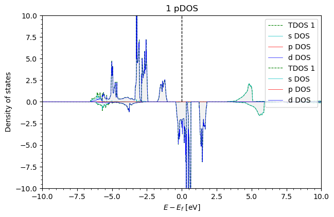
calc.get_pDOS()
FeCl2.pdos_atm#2(Cl)_wfc#2(p)
FeCl2.pdos_atm#2(Cl)_wfc#1(s)
FeCl2.pdos_atm#1(Fe)_wfc#1(s)
FeCl2.pdos_atm#3(Cl)_wfc#2(p)
FeCl2.pdos_atm#1(Fe)_wfc#4(d)
FeCl2.pdos_atm#1(Fe)_wfc#3(p)
FeCl2.pdos_atm#3(Cl)_wfc#1(s)
FeCl2.pdos_atm#1(Fe)_wfc#2(s)
[13]:
calc.plot_pDOS('1', efrom=-10, eto=10, yfrom=-10)
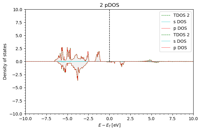
[14]:
calc.plot_pDOS('2', efrom=-10, eto=10, yfrom=-10)
Wannier bands
[15]:
calc.load_wannier(kpath_filename='kpath_qe2.dat', kpaths_dir='kpaths',
                     hr_up_name='hrup.dat', hr_dn_name='hrdn.dat')
nwa  11
Rpts 813
we have 3D hamiltonian
nwa  11
Rpts 813
we have 3D hamiltonian
100%|██████████| 116/116 [00:00<00:00, 194.86it/s]
100%|██████████| 116/116 [00:00<00:00, 193.26it/s]
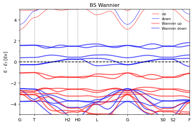
[16]:
#interpolate the bands, on the plot bolds are interpolated wannier bands
calc.plot_wannier_BS(efrom=-5, eto=5)
[17]:
#now we want to plot the wannier bands on several BZ (normally you don't need to do this)
# for 3D plot of isosurfaces

loader = wnldr.Wannier_loader_FM(hr_up_name='hrup.dat', hr_dn_name='hrdn.dat', wannier_dir='wannier')

acell = np.linalg.norm(calc.acell[0]) # AA
b1 = calc.bcell[0][:3] / (2. * np.pi / acell)  # First reciprocal lattice vector in units of 2pi/a
b2 = calc.bcell[1][:3] / (2. * np.pi / acell) # Second reciprocal lattice vector in units of 2pi/a
b3 = calc.bcell[2][:3] / (2. * np.pi / acell) # Third reciprocal lattice vector in units of 2pi/a
nwa  11
Rpts 813
we have 3D hamiltonian
nwa  11
Rpts 813
we have 3D hamiltonian
[ ]:
klim = 1.0 # want to have data in range [-1, 1] (in units of 2pi/a)
nkpt = 10

bs, _ = loader.get_dense_hk_symmetric(nkpt=nkpt, krange=klim, find_eigsQ=True)
[32]:
band_str_up = bs[:,:,0] # choose spin up
band_str_dn = bs[:,:,1]
[37]:
# k fractional
crystal_coords = np.mgrid[-klim:klim:1.0/nkpt, -klim:klim:1.0/nkpt, -klim:klim:1.0/nkpt].reshape(3,-1).T # repr cart in 2 pi / alat
crystal_coords = np.array(crystal_coords)
kx_cryst = crystal_coords[:, 0]
ky_cryst = crystal_coords[:, 1]
kz_cryst = crystal_coords[:, 2]


B = np.array([b1, b2, b3]).T  # Reciprocal lattice basis

cart_coords = np.dot(crystal_coords, B.T) #np.dot(B, crystal_coords.T)
# k cart (2 pi / alat)
kx_cart = cart_coords[:, 0]
ky_cart = cart_coords[:, 1]
kz_cart = cart_coords[:, 2]
[50]:
z = np.real(band_str_dn[ 7, :] - calc.efermi) # 7th band for example
print(np.max(z), np.min(z)) # check that fermi level is in the middle of the band
0.3289087332311933 -0.2727131988493481
[47]:
from scipy.interpolate import Rbf


# Create the RBF interpolator
rbf = Rbf(kx_cart, ky_cart, kz_cart, z, function='linear')

# Interpolate the values on the regular grid
# here _cryst coords stand for regular meshes in cartesian coordinates just because grid is the same
bs_cart_grid = rbf(kx_cryst, ky_cryst, kz_cryst)
[49]:
def get_brillouin_zone_3d(cell):
    """
    Uses the k-space vectors and voronoi analysis to define
    the BZ of the system

    Args:
        cell: a 3x3 matrix defining the basis vectors in
        reciprocal space

    Returns:
        vor.vertices[bz_vertices]: vertices of BZ
        bz_ridges: edges of the BZ
        bz_facets: BZ facets

    """

    px, py, pz = np.tensordot(cell, np.mgrid[-1:2, -1:2, -1:2], axes=[0, 0])
    points = np.c_[px.ravel(), py.ravel(), pz.ravel()]

    from scipy.spatial import Voronoi

    vor = Voronoi(points)

    bz_facets = []
    bz_ridges = []
    bz_vertices = []

    for pid, rid in zip(vor.ridge_points, vor.ridge_vertices):

        if pid[0] == 13 or pid[1] == 13:
            bz_ridges.append(vor.vertices[np.r_[rid, [rid[0]]]])
            bz_facets.append(vor.vertices[rid])
            bz_vertices += rid

    bz_vertices = list(set(bz_vertices))

    return vor.vertices[bz_vertices], bz_ridges, bz_facets
[48]:
vv = bs_cart_grid.flatten()

fig = go.Figure()

fig = go.Figure(data=go.Isosurface(
    x=kx_cryst,
    y=ky_cryst,
    z=kz_cryst,
    value=vv,
    isomin=-0.1,
    isomax=0.1,
    # surface_count=5, # number of isosurfaces, 2 by default: only min and max
    caps=dict(x_show=False, y_show=False)
    ))


fig.add_trace(go.Scatter3d(
    x=[0, b1[0], b2[0], b3[0]],
    y=[0, b1[1], b2[1], b3[1]],
    z=[0, b1[2], b2[2], b3[2]],
    mode='markers+text',
    marker=dict(size=5),
    text=['Origin', 'b1', 'b2', 'b3'],
    textposition='top center'
))

# Add arrows for each basis vector
for b in [b1, b2, b3]:
    fig.add_trace(go.Scatter3d(
        x=[0, b[0]],
        y=[0, b[1]],
        z=[0, b[2]],
        mode='lines',
        line=dict(color='green', width=5),
        showlegend=False
    ))

vertices, ridges, _ = get_brillouin_zone_3d(calc.bcell/ (2. * np.pi / acell))

# Plot vertices
fig.add_trace(go.Scatter3d(
    x=vertices[:, 0], y=vertices[:, 1], z=vertices[:, 2],
    mode='markers',
    marker=dict(size=5, color='red'),
    name='Vertices',
    showlegend=False
))

# Plot edges
for ridge in ridges:
    # points = vertices[ridge]

    fig.add_trace(go.Scatter3d(
        x=ridge[:, 0], y=ridge[:, 1], z=ridge[:, 2],
        mode='lines',
        line=dict(color='black', width=2),
        name='Edges',
    showlegend=False
    ))

# Show figure
fig.update_layout(
    title='3D Brillouin Zone',
    scene=dict(
        xaxis_title='kx',
        yaxis_title='ky',
        zaxis_title='kz'
    )
)

fig.show()
Data type cannot be displayed: application/vnd.plotly.v1+json
