3D PM Example
[1]:
%matplotlib inline
import numpy as np
import warnings
warnings.filterwarnings('ignore')
import plotly.graph_objects as go
[1]:
# import sys
# sys.path.append("../../src/")
[3]:
%load_ext autoreload
%autoreload 2

from qeview.qe_analyse_PM import qe_analyse_PM
import qeview.wannier_loader as wnldr
[4]:
Ang2Bohr = 1.8897259886
Bohr2Ang = 1./Ang2Bohr
QE Analysis
[6]:
calc = qe_analyse_PM('./', 'FeCl23D')
Unit Cell Volume:   64.1334  (Ang^3)
alat 6.4228
Reciprocal-Space Vectors cart (Ang^-1)
[[ 1.8467691455 -1.0662326633  0.327370275 ]
 [ 0.            2.1324653265  0.327370275 ]
 [-1.8467691455 -1.0662326633  0.327370275 ]]
Reciprocal-Space Vectors cart (2 pi / alat)
[[ 1.8877963546 -1.0899197335  0.3346430242]
 [ 0.            2.179839467   0.3346430242]
 [-1.8877963546 -1.0899197335  0.3346430242]]
Real-Space Vectors cart (Ang)
[[ 1.7011290563 -0.9821473186  6.3976336955]
 [ 0.            1.9642946371  6.3976336955]
 [-1.7011290563 -0.9821473186  6.3976336955]]
Real-Space Vectors cart (alat)
[[ 0.264859077  -0.1529164594  0.9960863047]
 [ 0.            0.3058329188  0.9960863047]
 [-0.264859077  -0.1529164594  0.9960863047]]


 positions cart (alat)
['Fe', 'Cl', 'Cl']
[[-0.           -0.           -0.          ]
 [ 0.           -0.            2.1814001212]
 [ 0.           -0.            0.8068587928]]
positions (frac or crystal)
[[-0.           -0.            0.          ]
 [ 0.7299903335  0.7299903335  0.7299903335]
 [ 0.2700096665  0.2700096665  0.2700096665]]
positions (AA)
[[-0.           -0.           -0.          ]
 [ 0.           -0.           14.0106322646]
 [ 0.           -0.            5.1822688218]]
[8]:
calc.get_band_structure(bands_filename='bands.dat.gnu', qe_dir='qe')
calc.get_sym_points(filename='band.in', qe_dir='qe')
[9]:
_,_ = calc.get_qe_kpathBS(filename="kpath_qe2.dat", saveQ=True, points_per_unit=20)
G 0.00000000 0.00000000 0.00000000 0.00000000
. 0.05000000 0.05000000 0.05000000 0.05019645
. 0.10000000 0.10000000 0.10000000 0.10039291
. 0.15000000 0.15000000 0.15000000 0.15058936
. 0.20000000 0.20000000 0.20000000 0.20078581
. 0.25000000 0.25000000 0.25000000 0.25098227
. 0.30000000 0.30000000 0.30000000 0.30117872
. 0.35000000 0.35000000 0.35000000 0.35137518
. 0.40000000 0.40000000 0.40000000 0.40157163
. 0.45000000 0.45000000 0.45000000 0.45176808
T 0.50000000 0.50000000 0.50000000 0.50196454
. 0.51324731 0.48675269 0.50000000 0.55198097
. 0.52649461 0.47350539 0.50000000 0.60199741
. 0.53974192 0.46025808 0.50000000 0.65201385
. 0.55298923 0.44701077 0.50000000 0.70203028
. 0.56623654 0.43376346 0.50000000 0.75204672
. 0.57948384 0.42051616 0.50000000 0.80206316
. 0.59273115 0.40726885 0.50000000 0.85207959
. 0.60597846 0.39402154 0.50000000 0.90209603
. 0.61922577 0.38077423 0.50000000 0.95211247
. 0.63247307 0.36752693 0.50000000 1.00212890
. 0.64572038 0.35427962 0.50000000 1.05214534
. 0.65896769 0.34103231 0.50000000 1.10216178
. 0.67221499 0.32778501 0.50000000 1.15217821
. 0.68546230 0.31453770 0.50000000 1.20219465
. 0.69870961 0.30129039 0.50000000 1.25221109
. 0.71195692 0.28804308 0.50000000 1.30222752
. 0.72520422 0.27479578 0.50000000 1.35224396
. 0.73845153 0.26154847 0.50000000 1.40226040
. 0.75169884 0.24830116 0.50000000 1.45227684
. 0.76494615 0.23505385 0.50000000 1.50229327
. 0.77819345 0.22180655 0.50000000 1.55230971
. 0.79144076 0.20855924 0.50000000 1.60232615
. 0.80468807 0.19531193 0.50000000 1.65234258
H2 0.81793537 0.18206463 0.50000000 1.70235902
. 0.76494615 0.12137642 0.44701077 1.76060311
. 0.71195692 0.06068821 0.39402154 1.81884721
. 0.65896769 0.00000000 0.34103231 1.87709130
. 0.60597846 -0.06068821 0.28804308 1.93533540
. 0.55298923 -0.12137642 0.23505385 1.99357949
H0 0.50000000 -0.18206463 0.18206463 2.05182359
. 0.50000000 -0.16805965 0.16805965 2.10470065
. 0.50000000 -0.15405468 0.15405468 2.15757772
. 0.50000000 -0.14004971 0.14004971 2.21045479
. 0.50000000 -0.12604474 0.12604474 2.26333185
. 0.50000000 -0.11203977 0.11203977 2.31620892
. 0.50000000 -0.09803480 0.09803480 2.36908599
. 0.50000000 -0.08402983 0.08402983 2.42196306
. 0.50000000 -0.07002486 0.07002486 2.47484012
. 0.50000000 -0.05601988 0.05601988 2.52771719
. 0.50000000 -0.04201491 0.04201491 2.58059426
. 0.50000000 -0.02800994 0.02800994 2.63347132
. 0.50000000 -0.01400497 0.01400497 2.68634839
L 0.50000000 0.00000000 0.00000000 2.73922546
. 0.47727273 0.00000000 0.00000000 2.78934765
. 0.45454545 0.00000000 0.00000000 2.83946985
. 0.43181818 0.00000000 0.00000000 2.88959205
. 0.40909091 0.00000000 0.00000000 2.93971424
. 0.38636364 0.00000000 0.00000000 2.98983644
. 0.36363636 0.00000000 0.00000000 3.03995863
. 0.34090909 0.00000000 0.00000000 3.09008083
. 0.31818182 0.00000000 0.00000000 3.14020303
. 0.29545455 0.00000000 0.00000000 3.19032522
. 0.27272727 0.00000000 0.00000000 3.24044742
. 0.25000000 0.00000000 0.00000000 3.29056961
. 0.22727273 0.00000000 0.00000000 3.34069181
. 0.20454545 0.00000000 0.00000000 3.39081401
. 0.18181818 0.00000000 0.00000000 3.44093620
. 0.15909091 0.00000000 0.00000000 3.49105840
. 0.13636364 0.00000000 0.00000000 3.54118059
. 0.11363636 0.00000000 0.00000000 3.59130279
. 0.09090909 0.00000000 0.00000000 3.64142499
. 0.06818182 0.00000000 0.00000000 3.69154718
. 0.04545455 0.00000000 0.00000000 3.74166938
. 0.02272727 0.00000000 0.00000000 3.79179157
G 0.00000000 0.00000000 0.00000000 3.84191377
. 0.01364129 -0.01364129 0.00000000 3.89341773
. 0.02728259 -0.02728259 0.00000000 3.94492170
. 0.04092388 -0.04092388 0.00000000 3.99642566
. 0.05456517 -0.05456517 0.00000000 4.04792963
. 0.06820646 -0.06820646 0.00000000 4.09943359
. 0.08184776 -0.08184776 0.00000000 4.15093756
. 0.09548905 -0.09548905 0.00000000 4.20244152
. 0.10913034 -0.10913034 0.00000000 4.25394549
. 0.12277163 -0.12277163 0.00000000 4.30544945
. 0.13641293 -0.13641293 0.00000000 4.35695342
. 0.15005422 -0.15005422 0.00000000 4.40845738
. 0.16369551 -0.16369551 0.00000000 4.45996134
. 0.17733680 -0.17733680 0.00000000 4.51146531
. 0.19097810 -0.19097810 0.00000000 4.56296927
. 0.20461939 -0.20461939 0.00000000 4.61447324
. 0.21826068 -0.21826068 0.00000000 4.66597720
. 0.23190197 -0.23190197 0.00000000 4.71748117
. 0.24554327 -0.24554327 0.00000000 4.76898513
. 0.25918456 -0.25918456 0.00000000 4.82048910
. 0.27282585 -0.27282585 0.00000000 4.87199306
. 0.28646714 -0.28646714 0.00000000 4.92349703
. 0.30010844 -0.30010844 0.00000000 4.97500099
. 0.31374973 -0.31374973 0.00000000 5.02650495
. 0.32739102 -0.32739102 0.00000000 5.07800892
S0 0.34103231 -0.34103231 0.00000000 5.12951288
. 0.39402154 -0.28419359 0.05683872 5.18591443
. 0.44701077 -0.22735488 0.11367744 5.24231597
. 0.50000000 -0.17051616 0.17051616 5.29871752
. 0.55298923 -0.11367744 0.22735488 5.35511907
. 0.60597846 -0.05683872 0.28419359 5.41152061
S2 0.65896769 0.00000000 0.34103231 5.46792216
. 0.64572038 0.00000000 0.35427962 5.51793859
. 0.63247307 0.00000000 0.36752693 5.56795503
. 0.61922577 0.00000000 0.38077423 5.61797147
. 0.60597846 0.00000000 0.39402154 5.66798790
. 0.59273115 0.00000000 0.40726885 5.71800434
. 0.57948384 0.00000000 0.42051616 5.76802078
. 0.56623654 0.00000000 0.43376346 5.81803721
. 0.55298923 0.00000000 0.44701077 5.86805365
. 0.53974192 0.00000000 0.46025808 5.91807009
. 0.52649461 0.00000000 0.47350539 5.96808652
. 0.51324731 0.00000000 0.48675269 6.01810296
F 0.50000000 0.00000000 0.50000000 6.06811940
[10]:
calc.plot_FullDOS(efrom=-10, eto=10)
Energies and DOS were not initialized. I run get_full_DOS
efermi 6.93

[11]:
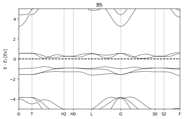
calc.plot_BS(efrom=-5, eto=5)
[12]:
calc.print_bands_range(7, 20)
efermi 6.93
-------------BANDS---------------
band 8 eV from  -0.18 to  1.15                 eV-eF from  -7.10 to  -5.77
band 9 eV from  -0.06 to  1.46                 eV-eF from  -6.99 to  -5.47
band 10 eV from  1.13 to  2.96                 eV-eF from  -5.79 to  -3.96
band 11 eV from  1.45 to  3.08                 eV-eF from  -5.48 to  -3.84
band 12 eV from  1.83 to  3.12                 eV-eF from  -5.09 to  -3.81
band 13 eV from  5.27 to  5.68                 eV-eF from  -1.66 to  -1.25
band 14 eV from  5.36 to  6.02                 eV-eF from  -1.57 to  -0.91
band 15 eV from  5.94 to  6.15                 eV-eF from  -0.98 to  -0.77
band 16 eV from  6.97 to  7.49                 eV-eF from  0.05 to  0.56
band 17 eV from  7.11 to  7.56                 eV-eF from  0.18 to  0.63
band 18 eV from  10.16 to  12.84                 eV-eF from  3.23 to  5.91
band 19 eV from  11.31 to  13.99                 eV-eF from  4.39 to  7.07
band 20 eV from  12.07 to  14.61                 eV-eF from  5.14 to  7.69
[13]:
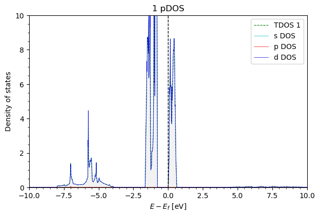
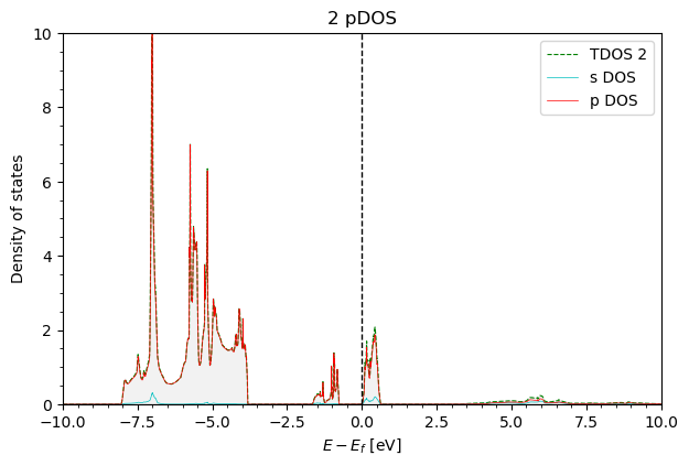
calc.get_pDOS()
FeCl23D.pdos_atm#1(Fe)_wfc#4(d)
FeCl23D.pdos_atm#1(Fe)_wfc#3(p)
FeCl23D.pdos_atm#3(Cl)_wfc#1(s)
FeCl23D.pdos_atm#3(Cl)_wfc#2(p)
FeCl23D.pdos_atm#2(Cl)_wfc#1(s)
FeCl23D.pdos_atm#1(Fe)_wfc#2(s)
FeCl23D.pdos_atm#1(Fe)_wfc#1(s)
FeCl23D.pdos_atm#2(Cl)_wfc#2(p)
[14]:
calc.plot_pDOS('1', efrom=-10, eto=10, yto=10)
[15]:
calc.plot_pDOS('2', efrom=-10, eto=10, yto=10)
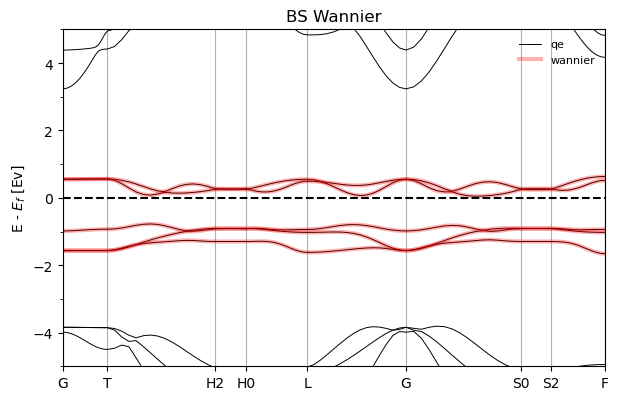
Wannier bands
[17]:
calc.load_wannier(kpath_filename='kpath_qe2.dat', wannier_hr_name='FeCl2_hr.dat')
nwa  5
Rpts 4391
we have 3D hamiltonian
100%|██████████| 119/119 [00:02<00:00, 44.32it/s]
[18]:
#interpolate the bands, on the plot bolds are interpolated wannier bands
calc.plot_wannier_BS(efrom=-5, eto=5)
[19]:
#now we want to plot the wannier bands on several BZ (normally you don't need to do this)
# for 3D plot of isosurfaces

loader = wnldr.Wannier_loader_PM('FeCl2_hr.dat', wannier_dir='wannier')

acell = np.linalg.norm(calc.acell[0]) # AA
b1 = calc.bcell[0][:3] / (2. * np.pi / acell)  # First reciprocal lattice vector in units of 2pi/a
b2 = calc.bcell[1][:3] / (2. * np.pi / acell) # Second reciprocal lattice vector in units of 2pi/a
b3 = calc.bcell[2][:3] / (2. * np.pi / acell) # Third reciprocal lattice vector in units of 2pi/a
nwa  5
Rpts 4391
we have 3D hamiltonian
[38]:
klim = 1.0 # want to have data in range [-1, 1] (in units of 2pi/a)
nkpt = 10

bs, _ = loader.get_dense_hk_symmetric(nkpt=nkpt, krange=klim, find_eigsQ=True)
100%|██████████| 8000/8000 [03:14<00:00, 41.19it/s]
[39]:
band_str = bs[:,:,0]
[40]:
# k fractional
crystal_coords = np.mgrid[-klim:klim:1.0/nkpt, -klim:klim:1.0/nkpt, -klim:klim:1.0/nkpt].reshape(3,-1).T # repr cart in 2 pi / alat
crystal_coords = np.array(crystal_coords)
kx_cryst = crystal_coords[:, 0]
ky_cryst = crystal_coords[:, 1]
kz_cryst = crystal_coords[:, 2]


B = np.array([b1, b2, b3]).T  # Reciprocal lattice basis

cart_coords = np.dot(crystal_coords, B.T) #np.dot(B, crystal_coords.T)
# k cart (2 pi / alat)
kx_cart = cart_coords[:, 0]
ky_cart = cart_coords[:, 1]
kz_cart = cart_coords[:, 2]
[48]:
z = np.real(band_str[ 3, :] - calc.efermi ) # 3th band for example
print(np.min(z), np.max(z) ) # check that fermi level is in the middle of the band
0.010464166457450297 0.560452231777461
[49]:
from scipy.interpolate import Rbf


# Create the RBF interpolator
rbf = Rbf(kx_cart, ky_cart, kz_cart, z, function='linear')

# Interpolate the values on the regular grid
# here _cryst coords stand for regular meshes in cartesian coordinates just because grid is the same
bs_cart_grid = rbf(kx_cryst, ky_cryst, kz_cryst)
[50]:
def get_brillouin_zone_3d(cell):
    """
    Uses the k-space vectors and voronoi analysis to define
    the BZ of the system

    Args:
        cell: a 3x3 matrix defining the basis vectors in
        reciprocal space

    Returns:
        vor.vertices[bz_vertices]: vertices of BZ
        bz_ridges: edges of the BZ
        bz_facets: BZ facets

    """

    px, py, pz = np.tensordot(cell, np.mgrid[-1:2, -1:2, -1:2], axes=[0, 0])
    points = np.c_[px.ravel(), py.ravel(), pz.ravel()]

    from scipy.spatial import Voronoi

    vor = Voronoi(points)

    bz_facets = []
    bz_ridges = []
    bz_vertices = []

    for pid, rid in zip(vor.ridge_points, vor.ridge_vertices):

        if pid[0] == 13 or pid[1] == 13:
            bz_ridges.append(vor.vertices[np.r_[rid, [rid[0]]]])
            bz_facets.append(vor.vertices[rid])
            bz_vertices += rid

    bz_vertices = list(set(bz_vertices))

    return vor.vertices[bz_vertices], bz_ridges, bz_facets
[51]:
vv = bs_cart_grid.flatten()

fig = go.Figure()

fig = go.Figure(data=go.Isosurface(
    x=kx_cryst,
    y=ky_cryst,
    z=kz_cryst,
    value=vv,
    isomin=0.2,
    isomax=0.4,
    # surface_count=5, # number of isosurfaces, 2 by default: only min and max
    caps=dict(x_show=False, y_show=False)
    ))


fig.add_trace(go.Scatter3d(
    x=[0, b1[0], b2[0], b3[0]],
    y=[0, b1[1], b2[1], b3[1]],
    z=[0, b1[2], b2[2], b3[2]],
    mode='markers+text',
    marker=dict(size=5),
    text=['Origin', 'b1', 'b2', 'b3'],
    textposition='top center'
))

# Add arrows for each basis vector
for b in [b1, b2, b3]:
    fig.add_trace(go.Scatter3d(
        x=[0, b[0]],
        y=[0, b[1]],
        z=[0, b[2]],
        mode='lines',
        line=dict(color='green', width=5),
        showlegend=False
    ))

vertices, ridges, _ = get_brillouin_zone_3d(calc.bcell/ (2. * np.pi / acell))

# Plot vertices
fig.add_trace(go.Scatter3d(
    x=vertices[:, 0], y=vertices[:, 1], z=vertices[:, 2],
    mode='markers',
    marker=dict(size=5, color='red'),
    name='Vertices',
    showlegend=False
))

# Plot edges
for ridge in ridges:
    # points = vertices[ridge]

    fig.add_trace(go.Scatter3d(
        x=ridge[:, 0], y=ridge[:, 1], z=ridge[:, 2],
        mode='lines',
        line=dict(color='black', width=2),
        name='Edges',
    showlegend=False
    ))

# Show figure
fig.update_layout(
    title='3D Brillouin Zone',
    scene=dict(
        xaxis_title='kx',
        yaxis_title='ky',
        zaxis_title='kz'
    )
)

fig.show()
Data type cannot be displayed: application/vnd.plotly.v1+json

[ ]: